The Ultimate Olympic Games Dashboard, visualising historical data about the modern olympic games 

Since the first COVID-19 vaccine was granted regulatory approval by the UK medicines regulator MHRA on December 2nd 2020, the question that has come across the mind of every brit has been whether or not they would take the vaccine against the coronavirus.The COVID-19 vaccine has become a primary focus for the government as it aims to increase the size of the vaccinated population. According to the UK Government, the percentage of those with at least one dose has increased from 60% on the 1st of May to 83.7% on the 1st of September. However, there is still a significant amount of people who have shown unwillingness or are vehemently refusing to take the vaccine.
This pool of people could become a problem to everyone as they may open the door for even more dangerous mutations than the delta variant and could eventually challenge the effectiveness of existing vaccines. So who are these people and how can the government try to address this issue with a data-driven approach?
The purpose of this project is to analyse the unvaccinated adult population in the United Kingdom, with a focus on how the government could potentially identify them so they can better plan their strategies to tackle the issue of vaccine hesitancy. Throughout the process, I also compare the rate of unvaccinated brits in different communities, areas and age groups.
For this analysis, I will be using the COVID-19 Behaviour Tracker survey made by Imperial College London and YouGov. The survey consists of fortnightly data from 29 countries around the world to explore the public’s attitudes and health behaviours as the situation evolves. I will be specifically looking at the United Kingdom data and attitudes towards the vaccine.
Before I state my approach, I will classify vaccine hesitancy for clarity. “Vaccine hesitancy” in the dataset I will explore refers to adults who:
Here’s a summary of my approach:
Now let’s start retrieving the data.
#imports
library(dplyr)
library(tidyr)
library(data.table)

#data
df <- read.csv('united-kingdom-data/united-kingdom.csv')
#head and tail of data
head(df)
tail(df)
| ï..RecordNo | endtime | qweek | i1_health | i2_health | i7a_health | i3_health | i4_health | i5_health_1 | i5_health_2 | ... | WAH5 | WAH7_1 | WAH7_2 | WAH7_3 | WAH7_4 | WAH7_5 | WAH7_6 | WAH7_7 | WAH7_99 | WAH6 | |
|---|---|---|---|---|---|---|---|---|---|---|---|---|---|---|---|---|---|---|---|---|---|
| <int> | <chr> | <chr> | <int> | <int> | <int> | <chr> | <chr> | <chr> | <chr> | ... | <chr> | <chr> | <chr> | <chr> | <chr> | <chr> | <chr> | <chr> | <chr> | <chr> | |
| 1 | 1921 | 01/04/2020 17:42 | week 1 | 3 | 2 | 1 | No, I have not | No, they have not | No | No | ... | ||||||||||
| 2 | 1922 | 01/04/2020 17:42 | week 1 | 3 | 0 | 2 | No, I have not | No, they have not | No | No | ... | ||||||||||
| 3 | 1923 | 01/04/2020 17:46 | week 1 | 1 | 12 | 1 | No, I have not | No, they have not | No | No | ... | ||||||||||
| 4 | 1924 | 01/04/2020 17:46 | week 1 | 1 | 2 | 1 | No, I have not | No, they have not | No | No | ... | ||||||||||
| 5 | 1925 | 01/04/2020 17:46 | week 1 | 2 | 0 | 1 | No, I have not | No, they have not | No | No | ... | ||||||||||
| 6 | 1926 | 01/04/2020 17:47 | week 1 | 0 | 0 | 0 | No, I have not | No, they have not | No | No | ... |
| ï..RecordNo | endtime | qweek | i1_health | i2_health | i7a_health | i3_health | i4_health | i5_health_1 | i5_health_2 | ... | WAH5 | WAH7_1 | WAH7_2 | WAH7_3 | WAH7_4 | WAH7_5 | WAH7_6 | WAH7_7 | WAH7_99 | WAH6 | |
|---|---|---|---|---|---|---|---|---|---|---|---|---|---|---|---|---|---|---|---|---|---|
| <int> | <chr> | <chr> | <int> | <int> | <int> | <chr> | <chr> | <chr> | <chr> | ... | <chr> | <chr> | <chr> | <chr> | <chr> | <chr> | <chr> | <chr> | <chr> | <chr> | |
| 52386 | 54305 | 07/10/2021 14:48 | week 51 | NA | 30 | NA | ... | Not very likely | |||||||||||||
| 52387 | 54309 | 07/10/2021 15:48 | week 51 | NA | 2 | NA | ... | Not at all likely | |||||||||||||
| 52388 | 54310 | 07/10/2021 16:15 | week 51 | NA | 1 | NA | ... | Not at all likely | |||||||||||||
| 52389 | 54125 | 07/10/2021 17:27 | week 51 | NA | 20 | NA | ... | Very likely | |||||||||||||
| 52390 | 54274 | 07/10/2021 21:56 | week 51 | NA | 5 | NA | ... | Not very likely | |||||||||||||
| 52391 | 54148 | 08/10/2021 08:15 | week 51 | NA | 10 | NA | ... | Very likely |
#structure of data
str(df)
'data.frame':	52391 obs. of  461 variables:
 $ ï..RecordNo       : int  1921 1922 1923 1924 1925 1926 1927 1928 1929 1930 ...
 $ endtime           : chr  "01/04/2020 17:42" "01/04/2020 17:42" "01/04/2020 17:46" "01/04/2020 17:46" ...
 $ qweek             : chr  "week 1" "week 1" "week 1" "week 1" ...
 $ i1_health         : int  3 3 1 1 2 0 6 0 2 4 ...
 $ i2_health         : int  2 0 12 2 0 0 10 0 0 0 ...
 $ i7a_health        : int  1 2 1 1 1 0 1 1 1 0 ...
 $ i3_health         : chr  "No, I have not" "No, I have not" "No, I have not" "No, I have not" ...
 $ i4_health         : chr  "No, they have not" "No, they have not" "No, they have not" "No, they have not" ...
 $ i5_health_1       : chr  "No" "No" "No" "No" ...
 $ i5_health_2       : chr  "No" "No" "No" "No" ...
 $ i5_health_3       : chr  "No" "No" "No" "No" ...
 $ i5_health_4       : chr  "No" "No" "No" "No" ...
 $ i5_health_5       : chr  "No" "No" "No" "No" ...
 $ i5_health_99      : chr  "Yes" "Yes" "Yes" "Yes" ...
 $ i5a_health        : chr  " " " " " " " " ...
 $ i6_health         : chr  " " " " " " " " ...
 $ i7b_health        : chr  " " " " " " " " ...
 $ i8_health         : chr  " " " " " " " " ...
 $ i9_health         : chr  "Yes" "Yes" "Yes" "Yes" ...
 $ i10_health        : chr  "Somewhat easy" "Very easy" "Very easy" "Somewhat difficult" ...
 $ i11_health        : chr  "Very willing" "Very willing" "Very willing" "Somewhat willing" ...
 $ i12_health_1      : chr  "Not at all" "Not at all" "Not at all" "Frequently" ...
 $ i12_health_2      : chr  "Always" "Always" "Always" "Always" ...
 $ i12_health_3      : chr  "Not at all" "Always" "Sometimes" "Frequently" ...
 $ i12_health_4      : chr  "Always" "Frequently" "Always" "Always" ...
 $ i12_health_5      : chr  "Not at all" "Sometimes" "Always" "Always" ...
 $ i12_health_6      : chr  "Frequently" "Sometimes" "Always" "Frequently" ...
 $ i12_health_7      : chr  "Not at all" "Not at all" "Always" "Always" ...
 $ i12_health_8      : chr  "Always" "Not at all" "Always" "Always" ...
 $ i12_health_9      : chr  "Always" "Not at all" "Always" "Not at all" ...
 $ i12_health_10     : chr  "Always" "Not at all" " " "Always" ...
 $ i12_health_11     : chr  "Always" "Always" "Not at all" "Always" ...
 $ i12_health_12     : chr  "Always" "Frequently" "Always" "Always" ...
 $ i12_health_13     : chr  "Always" "Frequently" "Always" "Always" ...
 $ i12_health_14     : chr  "Always" "Frequently" "Always" "Always" ...
 $ i12_health_15     : chr  "Always" "Always" "Always" "Always" ...
 $ i12_health_16     : chr  "Frequently" "Frequently" "Frequently" "Frequently" ...
 $ i12_health_17     : chr  "Not at all" "Not at all" "Always" "Not at all" ...
 $ i12_health_18     : chr  "Not at all" "Not at all" "Not at all" "Not at all" ...
 $ i12_health_19     : chr  "Sometimes" "Sometimes" "Always" "Always" ...
 $ i12_health_20     : chr  "Sometimes" "Rarely" "Always" "Always" ...
 $ i13_health        : int  17 25 20 20 6 10 8 20 10 8 ...
 $ i14_health_1      : chr  "No" "No" "No" "No" ...
 $ i14_health_2      : chr  "No" "No" "No" "No" ...
 $ i14_health_3      : chr  "No" "No" "No" "No" ...
 $ i14_health_4      : chr  "No" "Yes" "No" "No" ...
 $ i14_health_5      : chr  "No" "No" "No" "No" ...
 $ i14_health_6      : chr  "No" "No" "No" "No" ...
 $ i14_health_7      : chr  "No" "No" "No" "No" ...
 $ i14_health_8      : chr  "No" "No" "No" "No" ...
 $ i14_health_9      : chr  "No" "No" "No" "No" ...
 $ i14_health_10     : chr  "No" "No" "No" "No" ...
 $ i14_health_96     : chr  "No" "No" "No" "No" ...
 $ i14_health_98     : chr  "No" "No" "No" "No" ...
 $ i14_health_99     : chr  "Yes" "No" "Yes" "Yes" ...
 $ i14_health_other  : chr  "__NA__" "__NA__" "__NA__" "__NA__" ...
 $ d1_health_1       : chr  "No" "No" "No" "No" ...
 $ d1_health_2       : chr  "No" "No" "No" "No" ...
 $ d1_health_3       : chr  "No" "No" "No" "No" ...
 $ d1_health_4       : chr  "No" "No" "No" "No" ...
 $ d1_health_5       : chr  "No" "No" "No" "No" ...
 $ d1_health_6       : chr  "No" "No" "No" "No" ...
 $ d1_health_7       : chr  "No" "No" "No" "No" ...
 $ d1_health_8       : chr  "No" "No" "No" "No" ...
 $ d1_health_9       : chr  "No" "No" "No" "No" ...
 $ d1_health_10      : chr  "No" "No" "No" "No" ...
 $ d1_health_11      : chr  "No" "No" "No" "No" ...
 $ d1_health_12      : chr  "No" "No" "No" "No" ...
 $ d1_health_13      : chr  "No" "No" "No" "No" ...
 $ d1_health_98      : chr  "No" "No" "No" "No" ...
 $ d1_health_99      : chr  "Yes" "Yes" "Yes" "Yes" ...
 $ weight            : num  0.865 0.706 1.028 0.844 0.66 ...
 $ age               : int  37 43 45 33 39 30 38 58 64 28 ...
 $ region            : chr  "South East" "Scotland" "South East" "West Midlands" ...
 $ gender            : chr  "Male" "Male" "Female" "Female" ...
 $ household_size    : chr  "4" "3" "2" "2" ...
 $ household_children: chr  "2" "2" "0" "2" ...
 $ employment_status : chr  "Full time employment" "Full time employment" "Full time employment" "Full time employment" ...
 $ WCRex2            : chr  " " " " " " " " ...
 $ WCRV_4            : chr  " " " " " " " " ...
 $ CORE_B2_4         : chr  " " " " " " " " ...
 $ cantril_ladder    : int  NA NA NA NA NA NA NA NA NA NA ...
 $ PHQ4_1            : chr  " " " " " " " " ...
 $ PHQ4_2            : chr  " " " " " " " " ...
 $ PHQ4_3            : chr  " " " " " " " " ...
 $ PHQ4_4            : chr  " " " " " " " " ...
 $ m1_1              : chr  " " " " " " " " ...
 $ m1_2              : chr  " " " " " " " " ...
 $ m1_3              : chr  " " " " " " " " ...
 $ m1_4              : chr  " " " " " " " " ...
 $ m2                : int  NA NA NA NA NA NA NA NA NA NA ...
 $ m3                : int  NA NA NA NA NA NA NA NA NA NA ...
 $ m4_1              : chr  " " " " " " " " ...
 $ m4_2              : chr  " " " " " " " " ...
 $ m4_3              : chr  " " " " " " " " ...
 $ m4_4              : chr  " " " " " " " " ...
 $ m4_96             : chr  " " " " " " " " ...
 $ m4_99             : chr  " " " " " " " " ...
 $ m4_other          : chr  " " " " " " " " ...
  [list output truncated]
As shown, this is what the raw data looks like, it consists of 461 columns and 52391 rows. The entry of the records range from the dates April 2020 to October 2021. Alongside the survey questions and answers, the data also has some socioeconomic variables such as age, region, gender, employement status etc. The responses to the survey questions are categorical data which is useful too.
The survey questions in the data have been given aliases. To find out a description of the actual question, click here to view the accompanying document.
First, I will need to sort and filter the dataset.
For this analysis, I will be specifically looking at the unvaccinated adult population in the year 2021 and their attitudes and behaviour towards the vaccine. Therefore I need to:
I will also check for null records in the survey question columns and exclude those that do not answer any of the questions if need be as they would not be useful when performing analysis as well as making sure the data types are consistent with the nature of the data.
#changing variable data type
df$endtime <- as.Date(df$endtime,format="%d/%m/%Y")

#extracting month and year date values
df$year <- format(df$endtime,"%Y")

#filtering enteries from 2020
df <- filter(df,df$year == 2021)
Before I was able to filter by year, I needed to convert the data type from character to date and then extract the year from the date. Once I was able to do so, I proceeded to filter by the newly formed year variable.
# filtering the data for the unvaccinated respondents
df <- filter(df,vac =="No, neither")%>%filter(vac5=="No" | vac5 =="Not sure")
I have once again filtered the dataset to only include entries from the vaccine holdouts who, if the vaccine was avaliable to them, would not take it.
The variable ‘vac’ represents the question “Have you had the first or second doses of a Coronavirus (COVID-19) vaccine?” and the variable ‘vac5’ represents the question “If a Covid-19 vaccine is available to you, will you get it?”.
#irregular col name fix
df <-rename(df,RecordNo=ï..RecordNo)

# filtering out insignificant cols and spliting data into background and survey response data
df_background <- select(df,RecordNo,endtime,age,region,gender,household_size,household_children,employment_status,vac5)

#renaming variable vac5 in df_background for the sake of clarity
df_background <-rename(df_background,vac_willingness = vac5)
The data frame “df_background” consists of data relating to the respondents and the level of their vaccine hesitancy. Their willingness to get the vaccine will be used as a filter to try derive valuable insights when performing analysis.
# replace values to ensure data integrity
df_background$household_children <- replace(df_background$household_children,
                                            which(df_background$household_children=="7"),"5 or more")
I have noticed a data entry error. The valid values for the column ‘household_children’ are 0,1,2,3,4,5 or more and prefer not to say. There are many instances of two invalid entries, ‘7’ and ‘9’. I have replaced these values with the valid entry ‘5 or more’ as it fits the criteria.
#new age group variable
df_background$agegrp <- cut(df_background$age,breaks=c(18,25,35,45,55,65,Inf),
                            labels=c("18-24","25-34","35-45","45-55","55-65","65+"))
head(df_background,2)
| RecordNo | endtime | age | region | gender | household_size | household_children | employment_status | vac_willingness | agegrp | |
|---|---|---|---|---|---|---|---|---|---|---|
| <int> | <date> | <int> | <chr> | <chr> | <chr> | <chr> | <chr> | <chr> | <fct> | |
| 1 | 37046 | 2021-02-24 | 39 | London | Male | Don't know | 0 | Part time employment | Not sure | 35-45 |
| 2 | 37050 | 2021-02-24 | 71 | East Midlands | Female | 1 | 0 | Retired | Not sure | 65+ |
Finally, in the “df_background” dataframe I have made categorical variables for the continuous variable ‘age’. The intervals I have settled on for age are 18-24,25-34,35-44,45-54,55-64 and 65+.
#structure of data frame
str(df_background)
'data.frame':	339 obs. of  10 variables:
 $ RecordNo          : int  37046 37050 37058 37065 37071 37084 37090 37092 37124 37138 ...
 $ endtime           : Date, format: "2021-02-24" "2021-02-24" ...
 $ age               : int  39 71 28 42 42 39 66 41 49 50 ...
 $ region            : chr  "London" "East Midlands" "South East" "South West" ...
 $ gender            : chr  "Male" "Female" "Female" "Female" ...
 $ household_size    : chr  "Don't know" "1" "3" "3" ...
 $ household_children: chr  "0" "0" "0" "3" ...
 $ employment_status : chr  "Part time employment" "Retired" "Full time student" "Part time employment" ...
 $ vac_willingness   : chr  "Not sure" "Not sure" "No" "No" ...
 $ agegrp            : Factor w/ 6 levels "18-24","25-34",..: 3 6 2 3 3 3 6 3 4 4 ...
Looking at the dataset now, I have reduced the observations to 339 and we will be looking at 10 variables in the data frame. I am also satisfied that the data types for the corresponding variables are appropriate.
Let’s start analysing the data now.
I will start by performing some simple analysis and try notice if there are any interesting insights that can be taken away from in the background data.
#imports
library(modeest)
#crosstable
tbl_demographic <- df_background %>% group_by(vac_willingness) %>%
summarise(avg_age=round(mean(age),0),region=mfv(region),gender=mfv(gender),
          employment_status=mfv(employment_status),household_size=mfv(household_size),
          household_children=mfv(household_children),total_respondents=table(vac_willingness))

tbl_demographic
| vac_willingness | avg_age | region | gender | employment_status | household_size | household_children | total_respondents |
|---|---|---|---|---|---|---|---|
| <chr> | <dbl> | <chr> | <chr> | <chr> | <chr> | <chr> | <table> |
| No | 43 | North West | Female | Full time employment | 2 | 0 | 147 |
| Not sure | 40 | South East | Female | Full time employment | 2 | 0 | 192 |
I have created a cross table since I was working with many categorical variables and the results are interesting to say the least.
I will look now look closer at the variables: Region, Age group, Gender and Employment status.
#setting plot size
options(repr.plot.width=12, repr.plot.height=10)

#imports
library(sf)
library(geojsonio)
library(plotly)

#extracting datasets for regions and countries
eng <- geojson_read(paste0("https://opendata.arcgis.com/datasets/",
                              "8d3a9e6e7bd445e2bdcc26cdf007eac7_4.geojson"),
                                what="sp")
countries <- geojson_read(paste0("https://opendata.arcgis.com/datasets/",
                                   "92ebeaf3caa8458ea467ec164baeefa4_0.geojson"),
                                     what="sp")

#creating UK regions map data frame
eng <- st_as_sf(eng)
countries <- st_as_sf(countries)
UK <- countries[-1,]
names(eng)[3] <- "Region"
names(UK)[3] <- "Region"
UK$objectid <- 10:12
eng <- eng[-2]
UK <- UK[c(1, 3, 9:11)]
UK <- rbind(eng, UK)

#creating regions dataframe
data <- data.frame(table(df_background$region))

#renaming columns with appropriate names
data <-rename(data,Region=Var1)
data <-rename(data,Population=Freq)

#joining data
mapdata <- left_join(UK,data,by="Region")

#display
pl <- ggplot(mapdata, aes(fill = Population,label=Region)) + geom_sf() + geom_sf_text(colour = "black",size = 5,check_overlap = TRUE) +
        scale_fill_gradient(low = "blue",high="red") + ggtitle("Population of vaccine holdouts by Region") + theme_classic() +
         theme(axis.text = element_blank(), axis.ticks = element_blank(),axis.line = element_blank(),plot.margin = unit(c(0, 1, 0, 1), "cm")
          ,plot.title = element_text(size = 20, face = "bold"))

pl
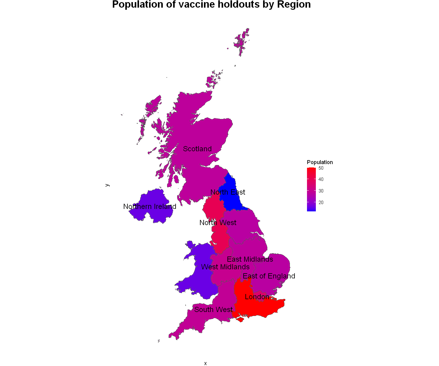
Looking at this map, we are capable of seeing the population level of all vaccine holdouts in the survey. We can see that the South East region is clearly the region with the most unvaccinated people in the UK, second would be the North West region and closely followed by London as the third most populated region.
On the other end of the scale, the North East, has the lowest total which is 12 people and both Wales and Northern Ireland have only 16 each.
There is also a high concentration of regions with a williingly unvaccinated population between 27-30 respondents.
We will now look at a plot dividing the population based on willingness level to see if we can get more interesting insights.
#setting plot size
options(repr.plot.width=8, repr.plot.height=8)

# imports
library(ggplot2)
library(treemapify)
library(grid)
library(gridExtra)

#aggregated dataframe
df_background_certain <- filter(df_background,vac_willingness=="No")
certain <- data.frame(table(df_background_certain$region))

df_background_uncertain <- filter(df_background,vac_willingness=="Not sure")
uncertain <- data.frame(table(df_background_uncertain$region))


# treemaps
pl_certain <- ggplot(data=certain,
       aes(x=Var1, fill=Var1, area=Freq,label=paste(Var1, Freq, sep="\n"),)) +
        geom_treemap() + geom_treemap_text(colour = "white", place = "centre",size = 15) +
         labs(title="Certain vaccine holdouts") + xlab("") +
          theme(legend.position = "none",axis.text.x = element_blank(),
           axis.ticks = element_blank())

pl_uncertain <- ggplot(data=uncertain,
       aes(x=Var1, fill=Var1, area=Freq,label=paste(Var1, Freq, sep="\n"),)) +
        geom_treemap() + geom_treemap_text(colour = "white", place = "centre",size = 15) +
         labs(title="Uncertain vaccine holdouts") + xlab("") +
          theme(legend.position = "none",axis.text.x = element_blank(),
           axis.ticks = element_blank())

#display
grid.arrange(pl_certain,pl_uncertain,ncol=1,nrow=2,top=textGrob(expression(bold("Population of vaccine holdouts by Region")),gp = gpar(col='black',fontsize=18)))
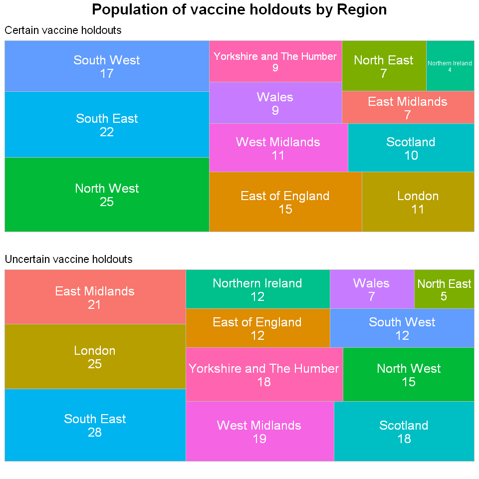
We can now gather more insightful takeaways from this treemap in addition to the geographical map. We can now see that the variance in the populations of each region. The one that stands out the most is the North West region. The majority of their vaccine holdouts, 60% of the unvaccinated population in the survey to be exact, are certain about not taking the vaccine which goes against the trend.
Another region with a huge differential between the uncertain and certain vaccine holdouts is London with an increase over 100% in uncertain vaccine holdouts compared to certain vaccine holdouts. East Midlands has increase of exactly 200%. These regions have shown the most potential for a high increase in vaccinated people.
The only region that appear in the top 3 in both charts is the South East region. Vaccine hesitancy is not really an issue in this region relative to the other regions.
# creating age dataframe
data.pl1 <- data.frame(df_background %>% select(agegrp,vac_willingness))
data.pl1 <- data.pl1[complete.cases(data.pl1),]

data.pl2 <- data.frame(df_background %>% select(agegrp))
data.pl2$status <- "Unvaccinated"
data.pl2 <- data.pl2[complete.cases(data.pl2),]

data.pl3 <-
#barplots
pl1 <- ggplot(data.pl1,aes(x=agegrp)) + geom_bar(aes(fill=vac_willingness),position="dodge") +
       labs(x ="",fill="Vaccine Willingness") + theme_classic()
pl2 <- ggplot(data.pl2,aes(x=agegrp)) + geom_bar(aes(fill=status)) +
       labs(x ="age group",fill="Vaccination status") + theme_classic()
pl3 <- ggplot(data.pl1,aes(x=agegrp)) + geom_bar(aes(fill=vac_willingness),position="fill") +
       labs(x ="",fill="Vaccine Willingness") + theme_classic()

#display
grid.arrange(pl1,pl3,pl2,top=textGrob(expression(bold("Population of vaccine holdouts distributed by Age")), gp = gpar(col='black',fontsize=18)))
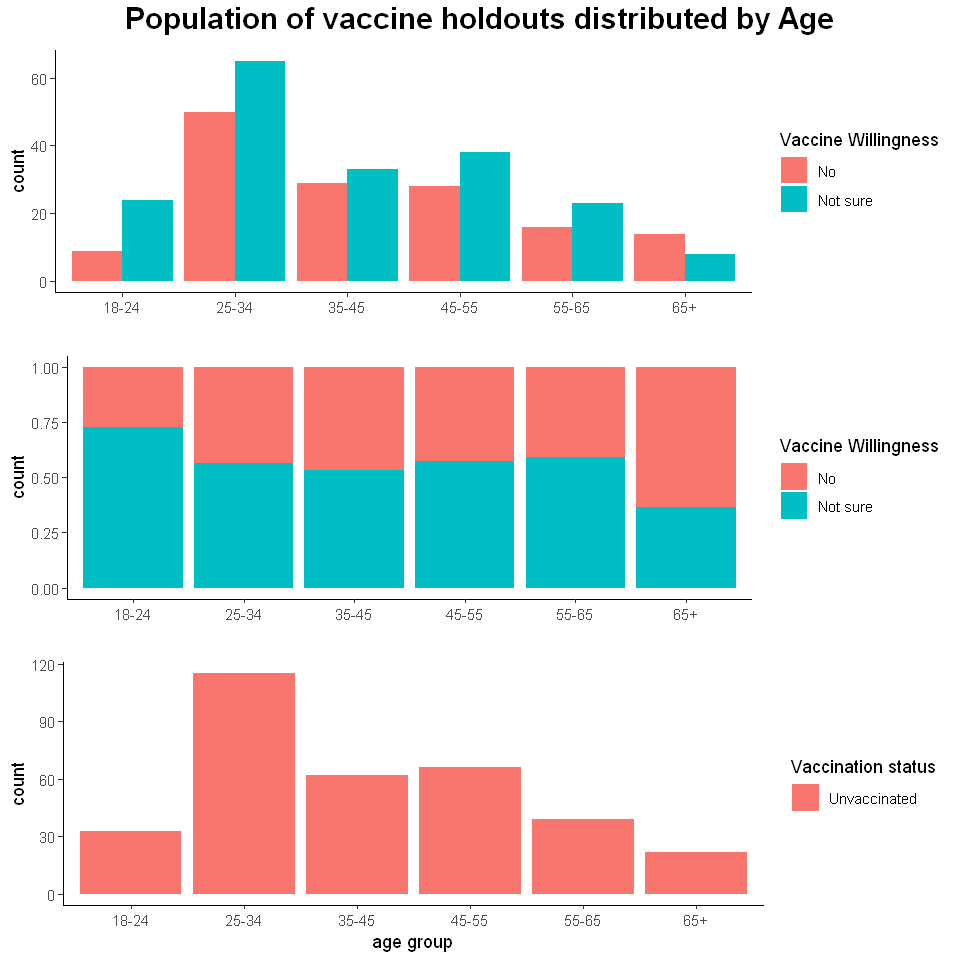
The first thing that standouts is that most unvaccinated respondents fall between the age range 25-34, which is far off the average age of approximately 40 years old that we gauged in our preliminary analysis. Therefore we can assume most unvaccinated people are in their late 20s going onto their early 30s.
There is also an outlier age group that does not follow the trend of more unsure vaccine holdouts to certain vaccine holdouts, which is 65+. There could be many reasons behind this outlier such as the vaccine was avaliable to the elderly for a longer time period in comparison to the other age groups so they would have had a lot more time to make a decision.
The government may instead want to focus its efforts on the young adults who are aged between 18-24 where the percentage of uncertain vaccine holdouts is approximately 75%, 3 times more in comparison to those who are certain about not taking the vaccine. There is a high potential to turn over the large majority of those who are uncertain about taking the vaccine.
#adjusting plot size
options(repr.plot.width=12, repr.plot.height=6)

#data function
df <- function(type){
#creating gender dataframe
df.gender <- df_background %>% select(gender,vac_willingness) %>% filter(gender==type)
data.gender <- data.frame(table(df.gender$vac_willingness,df.gender$gender))
data.gender$percentage <- (data.gender$Freq)/sum(data.gender$Freq)
data.gender$ymax = cumsum(data.gender$percentage)
data.gender$ymin = c(0, head(data.gender$ymax, n=-1))
data.gender$labelPosition <- (data.gender$ymax + data.gender$ymin) / 2
data.gender$label <- paste0(data.gender$Var1, "\n",round(data.gender$percentage*100,0),"%", "\n value: ", data.gender$Freq)
return(data.gender)
}
data.male <- df("Male")
data.female <- df("Female")

#creating dataframe for all genders
df.allgenders <- df_background %>% select(gender,vac_willingness)
df.allgenders$variable <- "All Genders"
data.allgenders <- data.frame(table(df.allgenders$vac_willingness,df.allgenders$variable))
data.allgenders$percentage <- (data.allgenders$Freq)/sum(data.allgenders$Freq)
data.allgenders$ymax = cumsum(data.allgenders$percentage)
data.allgenders$ymin = c(0, head(data.allgenders$ymax, n=-1))
data.allgenders$labelPosition <- (data.allgenders$ymax + data.allgenders$ymin) / 2
data.allgenders$label <- paste0(data.allgenders$Var1,"\n",round(data.allgenders$percentage*100,0),"%", "\n value: ", data.allgenders$Freq)

#combining dataframe
data.gender <- rbind(data.male,data.female,data.allgenders)

#donut charts
pl <- ggplot(data.gender, aes(ymax=ymax, ymin=ymin, xmax=4, xmin=3, fill=Var1)) +
        geom_rect() + geom_label( x=3.5, aes(y=labelPosition, label=label), size=4) +
          scale_fill_brewer(palette=18) + coord_polar(theta="y") + xlim(c(2, 4)) +
            theme_classic() + labs(title="Population of vaccine holdouts by Gender",x="",y="") + facet_grid(.~Var2) +
             theme(legend.position = "none", plot.title = element_text(size = 20),axis.text = element_blank(),
              axis.ticks = element_blank())
#display
pl
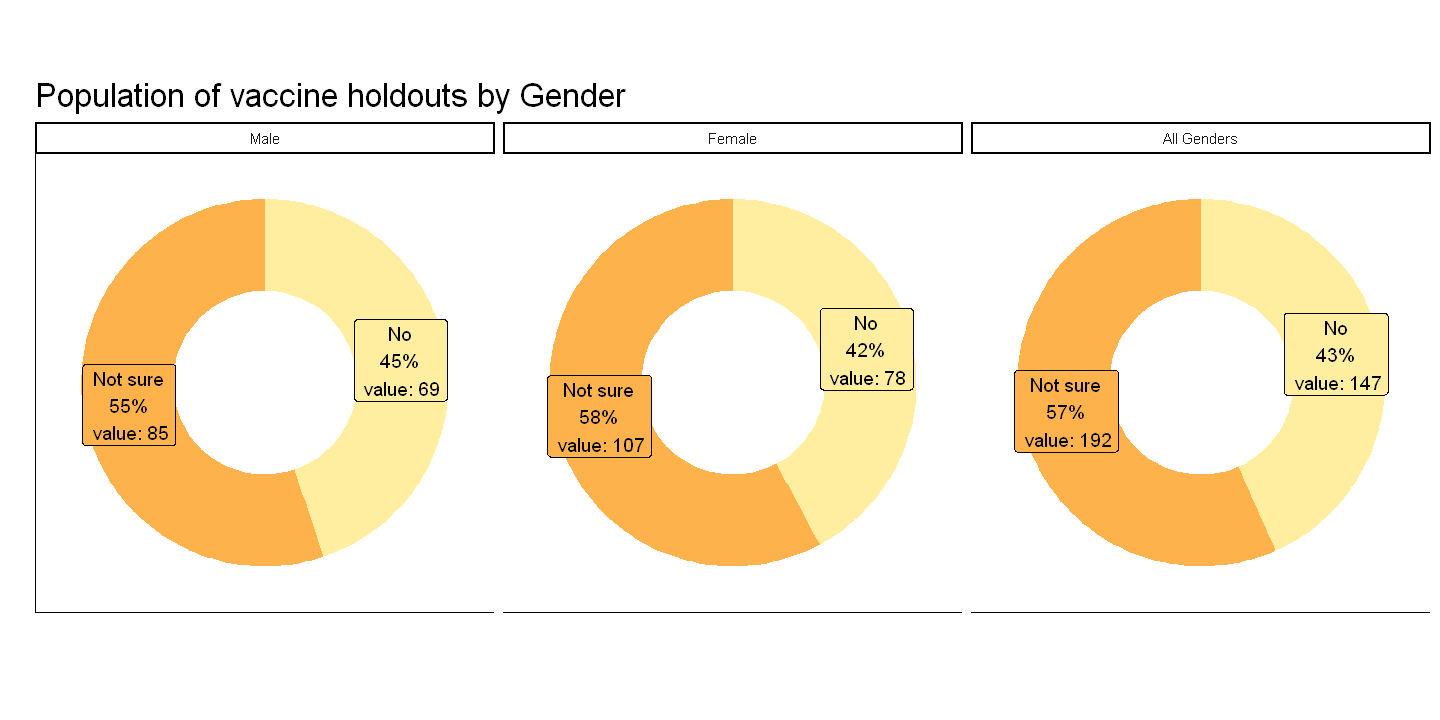
After observing the charts, we can see that the distribution between the two genders is very similar. They practically mirror the chart reflecting all genders. The relative change of the two charts range between 10-16%, which is very small.
The percentage of those who are unsure about taking the vaccine is greater amongst females in comparison to males. I would suggest to target more females however it is only greater by 3% which is virtually insignificant ao there are no significant insights that can be derived from this variable.
For the reasons I have stated, I would suggest not including gender as a factor for identifying vaccine holdouts and classifying them based on hesitancy level.
#adjusting plot size
options(repr.plot.width=12, repr.plot.height=8)

# imports
library(packcircles)

# plot function
plot <- function(status){
#data
d <- df_background %>% select(employment_status,vac_willingness) %>% filter(employment_status==status)
d <- data.frame(table(d$vac_willingness,group_by=d$employment_status))
d$percentage <- round(d$Freq/sum(d$Freq) * 100,0)

total <- sum(d$Freq)
packing <- circleProgressiveLayout(d$Freq, sizetype='area')
d <- cbind(d,packing)
data.gg <- circleLayoutVertices(packing, npoints=100)

#returning plot
return(ggplot() + geom_polygon(data = data.gg, aes(x, y, group = id, fill=as.factor(id)), colour = "black", alpha = 0.6) +
geom_text(data = d, aes(x, y, size=100,label= paste0(Var1,"\n",percentage,"%"))) +
  scale_size_continuous(range = c(1,10)) + theme_void() +
  theme(legend.position="none") + ggtitle(paste0(status,"\n","Total respondents: ",total)) +
  coord_equal())
       }

#Assigning plots by employment status
plot.FTE <- plot("Full time employment")
plot.PTE <- plot("Part time employment")
plot.FTS <- plot("Full time student")
plot.R <- plot("Retired")
plot.NW <- plot("Not working")
plot.U <- plot("Unemployed")

#creating plot grid
pl <- grid.arrange(plot.FTE,plot.PTE,plot.NW,plot.FTS,plot.R,plot.U,
             top=textGrob(expression(bold("Population of vaccine holdouts by Employment status")), gp = gpar(col='black',fontsize=20)))
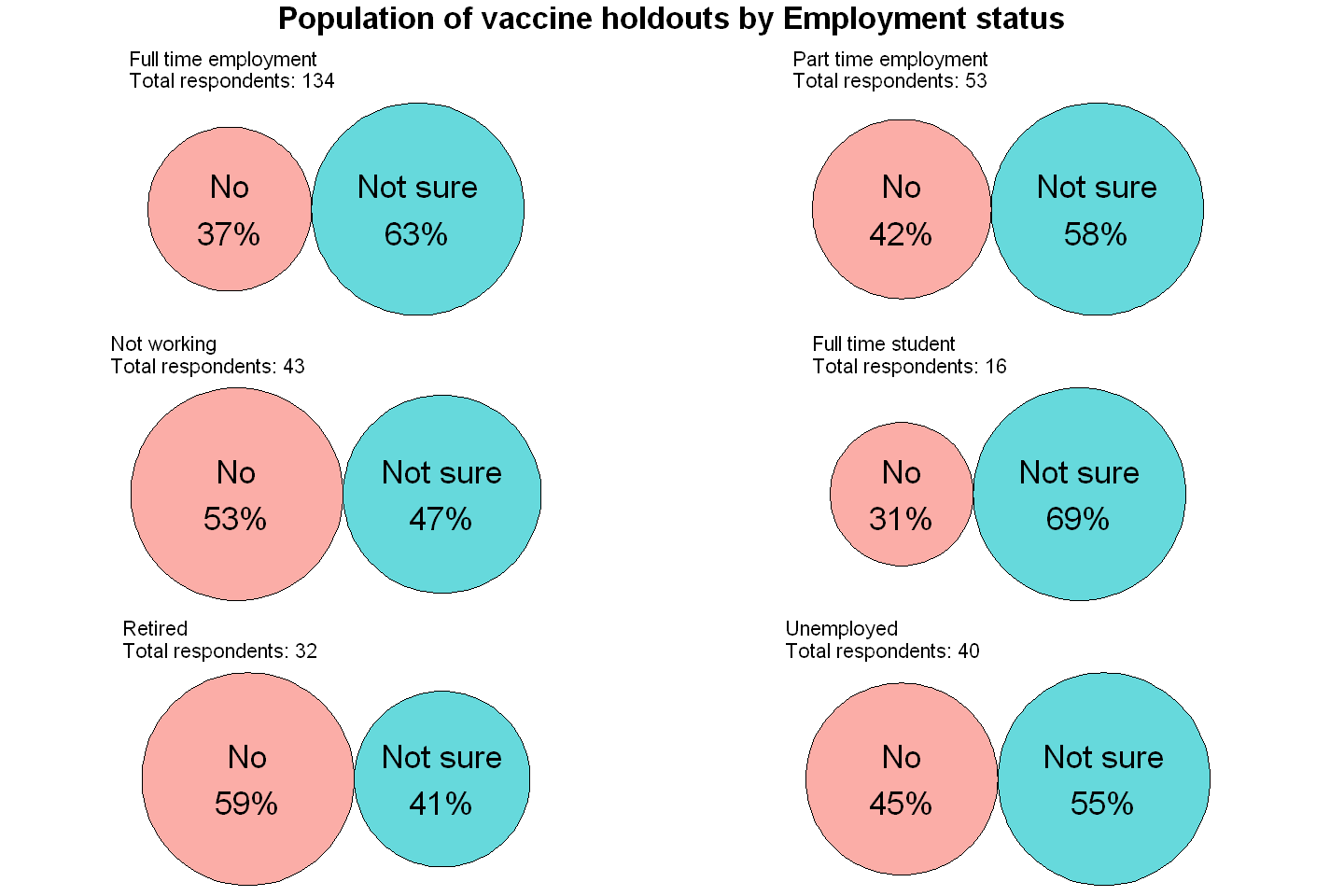
Once again, the reoccuring trend throughout the data has been broken. There is a far greater amount of people who firmly oppose taking the vaccine in comparison those who are uncertain about taking the vaccine amongst those who are retired. This follows another distinct trend which stems from the age variable.
d <- df_background %>% select(age,agegrp,employment_status) %>% #%>% filter(employment_status=="Retired")
      group_by(employment_status) %>% summarise(average.age=round(mean(age),0),age.group=mfv(agegrp))
d <- d %>% filter(employment_status != "Other")
d
| employment_status | average.age | age.group |
|---|---|---|
| <chr> | <dbl> | <fct> |
| Full time employment | 38 | 25-34 |
| Full time student | 24 | 18-24 |
| Not working | 44 | 45-55 |
| Part time employment | 40 | NA |
| Retired | 66 | 65+ |
| Unemployed | 36 | 25-34 |
Looking at this table now, we can see that the 65+ age group, which was the only age group that had more certain vaccine holdouts than uncertain vaccine holdouts, is predominantly represented by those who are retired, who also have a large amount of certain vaccine holdouts relative to uncertain vaccine holdouts.
Another interesting trend, the antithesis of the trend above, is that Full time students, which is predominantly represented by 18-24 year olds, have the largest percentage of unsure vaccine holdouts.
There seems to be a clear pattern amongst the demographic related variables.
Before I make any conclusions based on the analysis I have performed, I would like to talk about the assumptions that I have made with the survey data.
Based on the analysis, I have come to the conclusion that the government should be looking to mostly target the young adults in the age range of 18-24 years old who are predominantly full time students. They have shown to have the most upside potential in being able to convince to take the vaccine since those who have shown strong resistance to getting the vaccine are an underwhelming minority. The top 5 regions with the most uncertain vaccine holdouts are: South East, London, East Midlands, West Midlands and Yorkshire and The Humble. I would advise the government to also focus its efforts in those regions too.
In addition to the demographic to target, the one that has shown the most resistance to taking the vaccine is the elderly aged 65 years old or above and are retired. There could be many reasons behind this as stated earlier during the analysis, the vaccine was avaliable to the elderly for a longer time period in comparison to the other age groups so they would have had a lot more time to make a decision. This could mean the vaccinated elderly population have virtually reached its ceiling and expecting a huge change is unrealistic.
The golden era of cinema may have ended in the 1960s with the 5 major studios no longer being able to block book theaters by law after the paramount case, ho...
Since the first COVID-19 vaccine was granted regulatory approval by the UK medicines regulator MHRA on December 2nd 2020, the question that has come across t...